pacman::p_load(sf, sfdep, tmap, tidyverse)In-class Exercise 6: Spatial Weights and Applications
1.1 Overview
1.2 Getting Started
1.2.1 Installing and Loading the R Packages
1.3 The Data
1.3.1 Importing geospatial data
hunan <- st_read(dsn = "data/geospatial",
                 layer = "Hunan")
Reading layer `Hunan' from data source
`C:\valtyl\IS415-GAA\In-class_Ex\In-class_Ex06\data\geospatial'
using driver `ESRI Shapefile'
Simple feature collection with 88 features and 7 fields
Geometry type: POLYGON
Dimension: XY
Bounding box: xmin: 108.7831 ymin: 24.6342 xmax: 114.2544 ymax: 30.12812
Geodetic CRS: WGS 841.3.2 Importing attribute table
hunan2012 <- read_csv("data/aspatial/Hunan_2012.csv")1.3.3 Combining both data frame by using left join
hunan_GDPPC <- left_join(hunan, hunan2012) %>%
select(1:4, 7, 15)- note: to retain the geospatial properties, the left dataframe must be the sf dataframe (i.e. hunan)
- left_join() is from dplyr
- usually need to specific ‘join by what?’ but there is built in intelligence to identify which column exists in both
- to know which columns to select by, need to run hunan_GDPPC without the select statement first
1.3.4 Plotting a choropleth map
tmap_mode("plot")
tm_shape(hunan_GDPPC)+
  tm_fill("GDPPC",
          style = "quantile",
          palette = "Blues",
          title = "GDPPC") +
  tm_layout(main.title = "Distribution of GDP per capita by district, Hunan Province",
            main.title.position = "center",
            main.title.size = 1.0,
            legend.height = 0.40,
            legend.width = 0.30,
            frame = TRUE) +
  tm_borders(alpha = 0.5) +
  tm_compass(type="8star", size = 2) +
  tm_scale_bar() +
  tm_grid(alpha =0.2)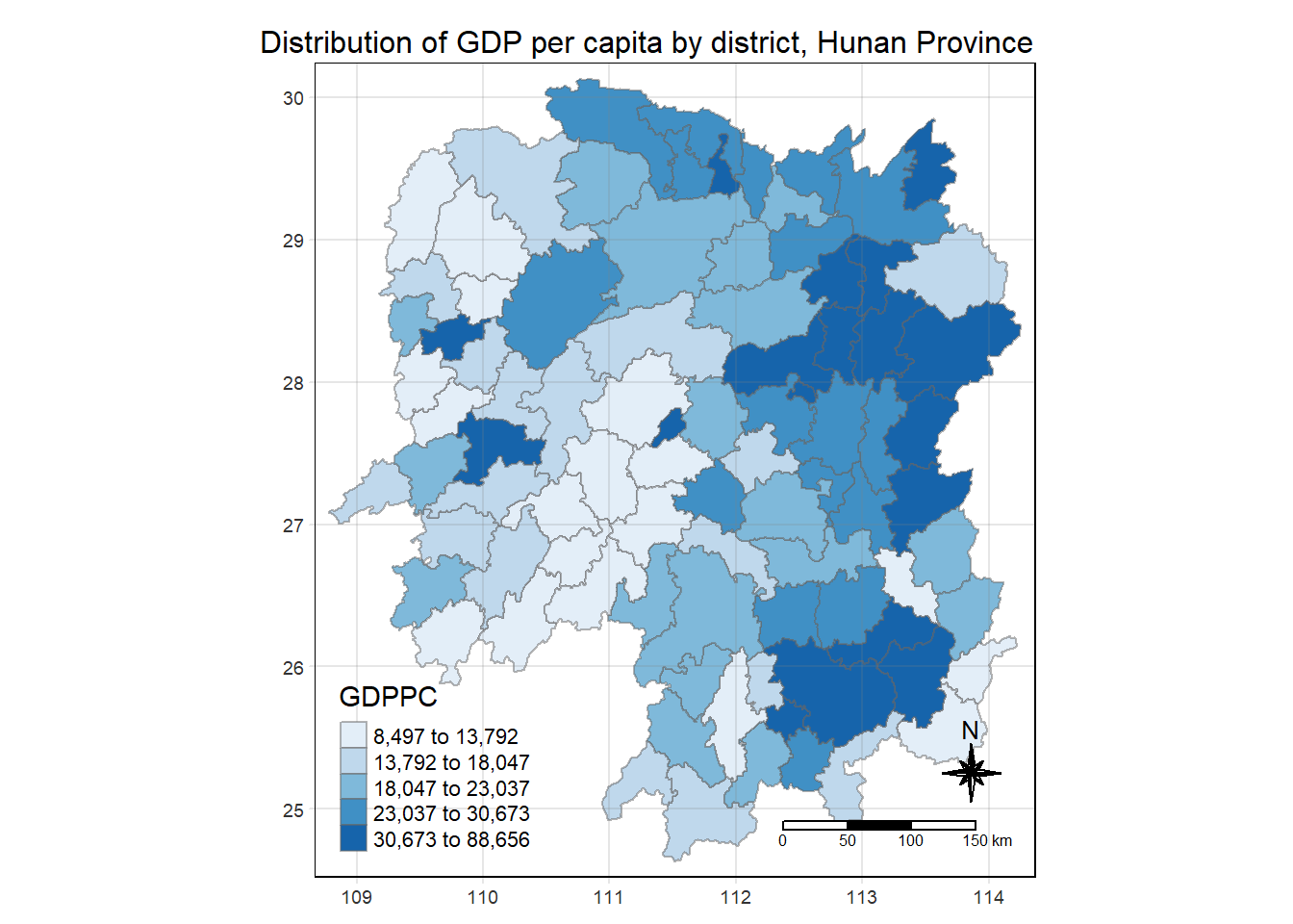
- default number of classes for the legend is 5
- alpha at the borders to reduce the intensity of the border
- classification method of quantile is acceptable, can explore other methods for other cases
1.4 Identify area neighbours
1.4.1 Contiguity neighbours method
Queen’s method
cn_queen <- hunan_GDPPC %>%
  mutate(nb = st_contiguity(geometry),
.before = 1)- more about st_contiguity()
- needs the geometry field of POLYGON sf dataframe
- chap 08 8.5.1,
poly2nb()is used from spdep, but here we are using sfdep - default is queen so dont need to state which method to use
hunan_GDPPCis sf polygon data and has the geometry columncn_queenretains the sf polygon and geometry attributes- .before=1 puts the newly created field at the first column of the table
Rook’s method
cn_rook <- hunan_GDPPC %>%
  mutate(nb = st_contiguity(geometry, queen = FALSE),
.before = 1)- spdep can do bishop method, sfdep cannot do bishop method
# geo <- sf_geometry()1.5 K-Nearest neighbours method
1.6 Distance band method
- sfdep st_dist_band
1.7 Computing contiguity weights
1.7.1 Contiguity weights: Queen’s method
wm_q <- hunan_GDPPC %>%
  mutate(nb = st_contiguity(geometry),
         wt = st_weights(nb),
.before = 1)- ^ this code combines 1.4.1 inside, so 1.4.1 is not needed
- the
wtcolumn of thewm_qoutput is now standardised
1.7.2 Contiguity weights: Rook’s method
wm_r <- hunan_GDPPC %>%
  mutate(nb = st_contiguity(geometry, queen = FALSE),
         wt = st_weights(nb),
.before = 1)queenhas to be placed beforewt